Mean, Median, and Mode – AEEFA SCHOOLS

Grade 8 – Mathematics

About Lesson

Mean

The arithmetic mean of a dataset (which is different from the geometric mean) is the sum of all values divided by the total number of values. It’s the most commonly used measure of central tendency because all values are used in the calculation.

Example: Finding the mean

Participant	1	2	3	4	5
Reaction time (milliseconds)	287	345	365	298	380

First you add up the sum of all values:

Then you calculate the mean using the formula

$begin{equation*} frac {sum{x}}{n} end{equation*}$

There are 5 values in the dataset, so n = 5.

$begin{equation*}bar{x}=dfrac{1,675}{5}=335end{equation*}$

Mean (x̄): 335 milliseconds

Outlier effect on the mean

Outliers can significantly increase or decrease the mean when they are included in the calculation. Since all values are used to calculate the mean, it can be affected by extreme outliers. An outlier is a value that differs significantly from the others in a dataset.

Example: In this dataset, we swap out one value with an extreme outlier.

Participant	1	2	3	4	5
Reaction time (milliseconds)	832	345	365	298	380

$begin{equation*}bar{x}=dfrac{sum{x}}{n}=dfrac{2,220}{5}=444end{equation*}$

Due to the outlier, the mean (x̄) becomes much higher, even though all the other numbers in the dataset stay the same.

Mean: 444 milliseconds

Population versus sample mean

A dataset contains values from a sample or a population. A population is the entire group that you are interested in researching, while a sample is only a subset of that population.

While data from a sample can help you make estimates about a population, only full population data can give you the complete picture.

In statistics, the notation of a sample mean and a population mean and their formulas are different. But the procedures for calculating the population and sample means are the same.

Sample mean formula

The sample mean is written as M or x̄ (pronounced x-bar). For calculating the mean of a sample, use this formula:

$begin{equation*}bar{x}=dfrac{sum{x}}{n}end{equation*}$

x̄: sample mean
$sum{x}$ : sum of all values in the sample dataset
n: number of values in the sample dataset

Population mean formula

The population mean is written as μ (Greek term mu). For calculating the mean of a population, use this formula:

$begin{equation*}mu=dfrac{sum{X}}{N}end{equation*}$

μ: population mean
$sum{X}$ : sum of all values in the population dataset
N: number of values in the population dataset

Median

The median of a dataset is the value that’s exactly in the middle when it is ordered from low to high.

Example: You measure the reaction times of 7 participants on a computer task and categorize them into 3 groups: slow, medium or fast.

Participant	1	2	3	4	5	6	7
Speed	Medium	Slow	Fast	Fast	Medium	Fast	Slow

To find the median, you first order all values from low to high. Then, you find the value in the middle of the ordered dataset—in this case, the value in the 4th position.

Ordered dataset	Slow	Slow	Medium	Medium	Fast	Fast	Fast

Median: Medium

In larger datasets, it’s easier to use simple formulas to figure out the position of the middle value in the distribution. You use different methods to find the median of a dataset depending on whether the total number of values is even or odd.

Median of an odd-numbered dataset

For an odd-numbered dataset, find the value that lies at the $dfrac{(n+1)}{2}$ position, where n is the number of values in the dataset.

Example: You measure the reaction times in milliseconds of 5 participants and order the dataset.

Reaction time (milliseconds)	287	298	345	365	380

The middle position is calculated using $dfrac{(n+1)}{2}$ , where n = 5.

$begin{equation*}dfrac{(5+1)}{2}=3$end{equation*}$

That means the median is the 3rd value in your ordered dataset.

Median: 345 milliseconds

Median of an even-numbered dataset

For an even-numbered dataset, find the two values in the middle of the dataset: the values at the $dfrac{n}{2}$ and $(dfrac{n}{2})+1$ positions. Then, find their mean.

Example: You measure the reaction times of 6 participants and order the dataset.

Reaction time (milliseconds)	287	298	345	357	365	380

The middle positions are calculated using $dfrac{n}{2}$ and $(dfrac{n}{2})+1$ , where n = 6.

$begin{equation*}dfrac{6}{2}=3end{equation*}$

$begin{equation*}(dfrac{6}{2})+1=4end{equation*}$

That means the middle values are the 3rd value, which is 345, and the 4th value, which is 357.

To get the median, take the mean of the 2 middle values by adding them together and dividing by 2.

$begin{equation*}dfrac{(345+357)}{2}=351end{equation*}$

Median: 351 milliseconds

Mode

The mode is the most frequently occurring value in the dataset. It’s possible to have no mode, one mode, or more than one mode.

To find the mode, sort your dataset numerically or categorically and select the response that occurs most frequently.

Example: In a survey, you ask 9 participants whether they identify as conservative, moderate, or liberal.

To find the mode, sort your data by category and find which response was chosen most frequently.

To make it easier, you can create a frequency table to count up the values for each category.

Political ideology	Frequency
Conservative	2
Moderate	3
Liberal	4

Mode: Liberal

When should you use the mean, median or mode?

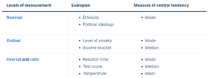
The 3 main measures of central tendency are best used in combination with each other because they have complementary strengths and limitations. But sometimes only 1 or 2 of them are applicable to your dataset, depending on the level of measurement of the variable.

The mode can be used for any level of measurement, but it’s most meaningful for nominal and ordinal levels.
The median can only be used on data that can be ordered – that is, from ordinal, interval and ratio levels of measurement.
The mean can only be used on interval and ratio levels of measurement because it requires equal spacing between adjacent values or scores in the scale.

Exercise Files

Mean_Median_Mode.pdf

Size: 2.11 MB